Postscript version of this file

STAT 450 Lecture 12

Reading for Today's Lecture: Chapter 4 section 4, Chapter 5 section 4.

Goals of Today's Lecture:

• Show that the mgf of a sum of independent quantities is the product of the individual mgfs.

• Evaluate some mgfs

• Use mgfs to find the $\chi^2_\nu$ density.

Last time: We defined

• For $X \in R$ the mgf (moment generating function) is
  
  $$M_X(t) = E(e^{tX}) \, .$$
  
  

• For $X\in R^p$ and $u \in R^p$ the mgf is
  
  $$M_X(u) = E[\exp{u^tX}] \, .$$
  
  

• The $r^{\rm th}$ moment (about the origin) of a real random variable X is $\mu_r^\prime=E(X^r)$. The $r^{\rm th}$ central moment is $\mu_r = E[(X-\mu)^r]$.

• The mgf is called that because
  
  $$M_X(t) = \sum_{k=0}^\infty \mu_k^\prime t^k/k!$$
  
  

Today's Notes

MGFs and Sums

If $X_1,\ldots,X_p$ are independent and $Y=\sum X_i$ then the moment generating function of Y is the product of those of the individual X_i:
$$\begin{align*}E(e^{tY}) & = \text{E}\left[e^{t \sum X_i}\right] \\ & = \text{E}\left[\prod e^{t X_i}\right] \\ & = \prod_i E(e^{tX_i}) \end{align*}$$
or $M_Y = \prod M_{X_i}$.

Cumulant generating functions and cumulants

NOTE: This section is extra material and will not be covered in class.

However this formula makes the power series expansion of M_Y not a particularly nice function of the expansions of the individual M_Xi. In fact this is related to the following observation. The first 3 moments (meaning $\mu$, $\sigma^2$ and $\mu_3$) of Y are just the sums of those of the X_i but this doesn't work for the fourth or higher moment.
$$\begin{align*}E(Y) =& \sum E(X_i) \\ {\rm Var}(Y) =& \sum {\rm Var}(X_i) \\ E[(Y-E(Y))^3] =& \sum E[(X_i-E(X_i))^3] \end{align*}$$
but
$$\begin{align*}E[(Y-E(Y))^4] =& \sum \{E[(X_i-E(X_i))^4] -E^2[(X_i-E(X_i))^2]\} \\ & + \left\{\sum E[(X_i-E(X_i))^2]\right\}^2 \end{align*}$$

It is possible, however, to replace the moments by other objects called cumulants which do add up properly. The way to define them relies on the observation that the log of the mgf of Y is the sum of the logs of the mgfs of the X_i. We define the cumulant generating function of a variable X by

$$K_X(t) = \log(M_X(t))$$

Then

$$K_Y(t) = \sum K_{X_i}(t)$$

The mgfs are all positive so that the cumulative generating functions are defined wherever the mgfs are. This means we can give a power series expansion of K_Y:

$$K_Y(t) = \sum_{r=1}^\infty \kappa_r t^r/r!$$

We call the $\kappa_r$ the cumulants of Y and observe

$$\kappa_r(Y) = \sum \kappa_r(X_i)$$

To see the relation between cumulants and moments proceed as follows: the cumulant generating function is
$$\begin{align*}K(t) &= \log(M(t)) \\ & = \log( 1 + [\mu_1 t +\mu_2^\prime t^2/2 + \mu_3^\prime t^3/3! + \cdots]) \end{align*}$$
To compute the power series expansion we think of the quantity in $[\ldots]$ as x and expand

$$\log(1+x) = x-x^2/2+x^3/3-x^4/4 \cdots \, .$$

When you stick in the power series

$$x=\mu t +\mu_2^\prime t^2/2 + \mu_3^\prime t^3/3! + \cdots$$

you have to expand out the powers of x and collect together like terms. For instance,
$$\begin{align*}x^2 &= \mu^2 t^2 + \mu\mu_2^\prime t^3 + [2\mu_3^\prime \mu/3! +(\... ...3 + 3\mu_2^\prime \mu^2 t^4/2 + \cdots \\ x^4 = \mu^4 t^4 + \cdots \end{align*}$$
Now gather up the terms. The power t¹ occurs only in x with coefficient $\mu$. The power t² occurs in x and in x² and so on. Putting these together gives
$$\begin{align*}K(t) =& \mu t \\ & + [\mu_2^\prime -\mu^2]t^2/2 \\ & + [\mu_3^\p... ... -3(\mu_2^\prime)^2 + 12 \mu_2^\prime \mu^2 -6\mu^4]t^4/4! + \cdots \end{align*}$$
Comparing coefficients of t^r/r! we see that
$$\begin{align*}\kappa_1 &= \mu \\ \kappa_2 &= \mu_2^\prime -\mu^2=\sigma^2 \\ \... ...ime)^2 + 12 \mu_2^\prime \mu^2 -6\mu^4 \\ &= E[(X-\mu)^4]-3\sigma^4 \end{align*}$$

Check the book by Kendall and Stuart (or the new version called Kendall's Theory of Statistics by Stuart and Ord) for formulas for larger orders r.

Example: If $X_1,\ldots,X_p$ are independent and X_i has a $N(\mu_i,\sigma^2_i)$ distribution then
$$\begin{align*}M_{X_i}(t) = &\int_{-\infty}^\infty e^{tx} e^{-(x-\mu_i)/\sigma_i^... ...2+t^2\sigma_i^2/2} dz/\sqrt{2\pi} \\ =& e^{\sigma_i^2t^2/2+t\mu_i} \end{align*}$$

This makes the cumulant generating function

$$K_{X_i}(t) = \log(M_{X_i}(t)) = \sigma_i^2t^2/2+\mu_i t$$

and the cumulants are $\kappa_1=\mu_i$, $\kappa_2=\sigma_i^2$ and every other cumulant is 0. The cumulant generating function for $Y=\sum X_i$ is

$$K_Y(t) = \sum \sigma_i^2 t^2/2 + t \sum \mu_i$$

which is the cumulant generating function of $N(\sum \mu_i,\sum\sigma_i^2)$.

NOTE: End of extra material.

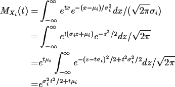
Example: I am having you derive the moment generating function of a Gamma rv. Suppose that $Z_1,\ldots,Z_\nu$ are independent N(0,1) rvs. Then we have defined $S_\nu = \sum_1^\nu Z_i^2$ to have a $\chi^2$distribution. It is easy to check S₁=Z₁² has density

$$(u/2)^{-1/2} e^{-u/2}/(2\sqrt{\pi})$$

and then the mgf of S₁ is

$$(1-2t)^{-1/2} \, .$$

It follows that

$$M_{S_\nu}(t) = (1-2t)^{-\nu/2};$$

you will show in homework that this is the mgf of a Gamma$(\nu/2,2)$ rv. This shows that the $\chi^2_\nu$ distribution has the Gamma$(\nu/2,2)$ density which is

$$(u/2)^{(\nu-2)/2}e^{-u/2} / (2\Gamma(\nu/2)) \, .$$

Example: The Cauchy density is

$$\frac{1}{\pi(1+x^2)}$$

and the corresponding moment generating function is

$$M(t) = \int_{-\infty}^\infty \frac{e^{tx}}{\pi(1+x^2)} dx$$

which is $+\infty$ except for t=0 where we get 1. This mgf is exactly the mgf of every t distribution so it is not much use for distinguishing such distributions. The problem is that these distributions do not have infinitely many finite moments.

This observation has led to the development of a substitute for the mgf which is defined for every distribution, namely, the characteristic function.

Characteristic Functions

NOTE: The material in this section is extra; I will not be covering it in 450.

Definition: The characteristic function of a real rv X is

$$\phi_X(t) = E(e^{itX})$$

where $i=\sqrt{-1}$ is the imaginary unit.

Aside on complex arithmetic.

The complex numbers are the things you get if you add $i=\sqrt{-1}$ to the real numbers and require that all the usual rules of algebra work. In particular if i and any real numbers a and b are to be complex numbers then so must be a+bi. If we multiply a complex number a+bi with a and b real by another such number, say c+di then the usual rules of arithmetic (associative, commutative and distributive laws) require
$$\begin{align*}(a+bi)(c+di)= & ac + adi+bci+bdi^2 \\ = & ac +bd(-1) +(ad+bc)i \\ =& (ac-bd) +(ad+bc)i \end{align*}$$
so this is precisely how we define multiplication. Addition is simply (again by following the usual rules)

(a+bi)+(c+di) = (a+b)+(c+d)i

Notice that the usual rules of arithmetic then don't require any more numbers than things of the form

x+yi

where x and y are real. We can identify a single such number x+yi with the corresponding point (x,y) in the plane. It often helps to picture the complex numbers as forming a plane.

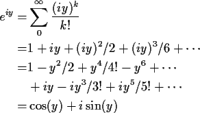
Now look at transcendental functions. For real x we know $e^x = \sum x^k/k!$ so our insistence on the usual rules working means

e^x+iy = e^x e^iy

and we need to know how to compute e^iy. Remember in what follows that i²=-1 so i³=-i, i⁴=1 i⁵=i¹=i and so on. Then
$$\begin{align*}e^{iy} =& \sum_0^\infty \frac{(iy)^k}{k!} \\ = & 1 + iy + (iy)^2/... ...ots \\ & + iy -iy^3/3! +iy^5/5! + \cdots \\ =& \cos(y) +i\sin(y) \end{align*}$$
We can thus write

$$e^{x+iy} = e^x(\cos(y)+i\sin(y))$$

Now every point in the plane can be written in polar co-ordinates as $(r\cos\theta, r\sin\theta)$ and comparing this with our formula for the exponential we see we can write

$$x+iy = \sqrt{x^2+y^2} e^{i\theta}$$

for an angle $\theta\in[0,2\pi)$.

We will need from time to time a couple of other definitions:

Definition: The modulus of the complex number x+iy is

$$\vert x+iy\vert = \sqrt{x^2+y^2}$$

Definition: The complex conjugate of x+iy is $\overline{x+iy} = x-iy$.

Notes on calculus with complex variables. Essentially the usual rules apply so, for example,

$$\frac{d}{dt} e^{it} = ie^{it}$$

We will (mostly) be doing only integrals over the real line; the theory of integrals along paths in the complex plane is a very important part of mathematics, however.

End of Aside

Since

$$e^{itX} = \cos(tX) + i \sin(tX)$$

we find that

$$\phi_X(t) = E(\cos(tX)) + i E(\sin(tX))$$

Since the trigonometric functions are bounded by 1 the expected values must be finite for all t and this is precisely the reason for using characteristic rather than moment generating functions in probability theory courses.

End of extra material.

Theorem For any two real rvs X and Y the following are equivalent:

1.

X and Y have the same distribution, that is, for any (Borel) set A we have

$$P(X\in A) = P( Y \in A)$$

2.

F_X(t) = F_Y(t) for all t.

3.

$\phi_X=E(e^{itX}) = E(e^{itY}) = \phi_Y(t)$ for all real t.

Moreover, all of these are implied if there is a positive $\epsilon$ such that for all $\vert t\vert \le \epsilon$

$$M_X(t)=M_Y(t) < \infty\,.$$