Goals of Today's Lecture:
Today's notes
Up to now we have tried to compute the density or cdf of some transformation, Y=g(X), of the data X exactly. In most cases this is not possible. Instead theoretical statisticians try to find methods to compute fY or FY approximately. There are really two standard methods:
In this course we focus on large sample theory.
You already know two large sample theorems:

I want to make these theorems precise (though I don't intend to prove them convincingly). I want you to have a good intuitive grasp of the meanings of the assertions, however.
There are two different senses in which
![]() :
convergence in probability and almost sure convergence.
:
convergence in probability and almost sure convergence.
Definition: A sequence Yn of random variables converges in probability
to Y if, for each
![]() :
:
Definition: A sequence Yn of random variables converges almost
surely (or strongly) to Y if
Notice that the second kind of convergence asks to to calculate a single
probability -- of an event whose definition is very complicated since
it mentions all the Yn at the same time. The first kind of
convergence involves computing a sequence of probabilities. The nth
probability in the sequence mentions only 2 random variables, Yn and
Y. Typically convergence in probability is easier to prove; it is
a theorem that ![]() almost surely implies
almost surely implies ![]() in
probability. (Notice the way we write those assertions.)
in
probability. (Notice the way we write those assertions.)
Corresponding to the two kinds of convergence are two precise versions of the law of large numbers:
Theorem: the Weak Law of Large Numbers. If
![]() are independent and identically distributed
random variables such that
are independent and identically distributed
random variables such that
![]() then the sequence of sample means,
then the sequence of sample means,

Theorem: the Strong Law of Large Numbers. If
![]() are independent and identically distributed
random variables such that
are independent and identically distributed
random variables such that
![]() then the sequence of sample means,
then the sequence of sample means,

The SLLN (note the abbreviation) is harder to prove. The WLLN
can be deduced, provided
![]() from
Chebyshev's inequality:
from
Chebyshev's inequality:
Chebyshev's inequality: If
![]() then
then
To apply the theorem let
![]() be independent and
identically distributed (iid) with mean
be independent and
identically distributed (iid) with mean ![]() and variance
and variance ![]() .
Then
.
Then ![]() has mean
has mean ![]() and
and
![]() .
Thus
.
Thus

This is a sort of approximate distribution calculation. We say that
a certain random variable has almost the same distribution as another,
namely, if n is large then the random variable ![]() has almost
the same distribution as the (nonrandom) quantity
has almost
the same distribution as the (nonrandom) quantity ![]() .
.
In some of the calculations we are about to make that
approximation is good enough. In others, however, we want to know
just how close to ![]() the quantity
the quantity ![]() is likely to be.
The answer is provided by the central limit theorem.
is likely to be.
The answer is provided by the central limit theorem.
If
![]() are iid with mean 0 and variance 1 then
are iid with mean 0 and variance 1 then
![]() converges in distribution to N(0,1). In previous
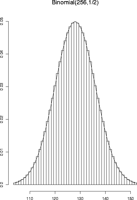
textbooks you will have seen pictures like the following:
converges in distribution to N(0,1). In previous
textbooks you will have seen pictures like the following:

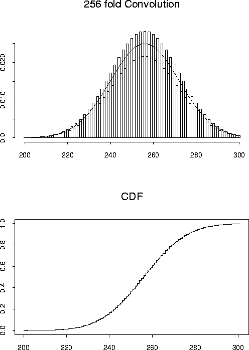
Here is another example of the central limit theorem. Here
the Xi are independent and identically distributed random variables
with
P(Xi=0)=P(Xi=2)=127.5/256 and
P(Xi=1)=1/256. The
top plot shows a histogram style plot of
![]() against k. The variable Y has mean 128 and standard deviation
against k. The variable Y has mean 128 and standard deviation
![]() .
You are meant to see that the superimposed
normal curve goes between the odd number bars and the even number bars.
.
You are meant to see that the superimposed
normal curve goes between the odd number bars and the even number bars.
The plots illustrate the difference between the local central
limit theorem, which says that the density of ![]() is close
to the normal density and the global central limit theorem
which says that the cdf of
is close
to the normal density and the global central limit theorem
which says that the cdf of ![]() is close
to the normal cdf.
That is,
is close
to the normal cdf.
That is,

 <\CENTER>

In this course we will state (but not really prove) a number of theorems with conclusions of this form. To do so we need some mathematical tools.
If
![]() are iid from a population with mean
are iid from a population with mean ![]() and standard
deviation
and standard
deviation ![]() then
then
![]() has approximately
a normal distribution. We also say that a Binomial(n,p) random variable
has approximately a
N(np,np(1-p)) distribution.
has approximately
a normal distribution. We also say that a Binomial(n,p) random variable
has approximately a
N(np,np(1-p)) distribution.
To make precise sense of these assertions we need to assign a meaning to
statements like ``X and Y have approximately the same distribution''.
The meaning we want to give is that X and Y have nearly the same cdf
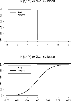
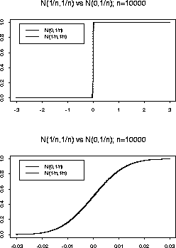
but even here we need some care. If n is a large number is the
N(0,1/n) distribution close to the distribution of ![]() ? Is it
close to the
N(1/n,1/n) distribution? Is it close to the
? Is it
close to the
N(1/n,1/n) distribution? Is it close to the
![]() distribution? If
distribution? If
![]() is the distribution
of Xn close to that of
is the distribution
of Xn close to that of ![]() ?
?
The answer to these questions depends in part on how close close needs to be so it's a matter of definition. In practice the usual sort of approximation we want to make is to say that some random variable X, say, has nearly some continuous distribution, like N(0,1). In this case we must want to calculate probabilities like P(X>x) and know that this is nearly P(N(0,1) > x). The real difficulty arises in the case of discrete random variables; in this course we will not actually need to approximate a distribution by a discrete distribution.
When mathematicians say two things are close together they either can provide an upper bound on the distance between the two things or they are talking about taking a limit. In this course we do the latter.
Definition: A sequence of random variables Xn converges in
distribution to a random variable X if
Theorem: The following are equivalent:
Now let's go back to the questions I asked:


Here is the message you are supposed to take away from this discussion. You do distributional approximations by showing that a sequence of random variables Xn converges to some X. The limit distribution should be non-trivial, like say N(0,1). We don't say Xn is approximately N(1/n,1/n) but that n1/2 Xn converges to N(0,1) in distribution.