Postscript version of these notes

STAT 350: Lecture 17

Reading: There is no truly relevant part of the text except chapter 5.

Summary of Last Time:

Suppose

$$X = \left[\begin{array}{c} X_1 \\ \hline X_2 \end{array}\righ... ..._{12} \\ \Sigma_{21} & \Sigma_{22} \end{array}\right]\right)$$

Then

1.

The covariance between X₁ and X₂ is

$$\Sigma_{12}= {\rm E}[(X_1-\mu_1)(X_2-\mu_2)^T] \equiv {\rm Cov}(X_1,X_2)$$

2.

$\Sigma_{12}=0 \Leftrightarrow \mbox{$X_1$\space independent of $X_2$ }$

3.

In the regression model $Y=X\beta+\epsilon$ with $\epsilon\sim MVN(0,\sigma^2 I)$

$$\left[ \begin{array}{c} \hat\mu \\ \hline \hat\epsilon \end{a... ...t[ \begin{array}{cc} H & 0 \\ 0 & I-H\end{array}\right]\right)$$

so that $\hat\mu$ and $\hat\epsilon$ are independent.

4.

It follows that the Regression Sum of Squares (unadjusted) (= $\hat\mu\hat\mu$) and the Error Sum of Squares (= $\hat\epsilon^T \hat\epsilon$) are independent.

5.

Similarly

$$\left[ \begin{array}{c} \hat\beta \\ \hline \hat\epsilon \end... ...array}{cc} (X^TX)^{-1} & 0 \\ 0 & I-H\end{array}\right]\right)$$

so that $\hat\beta$ and $\hat\epsilon$ are independent.

Conclusion:

$$a^T\hat\beta - a^T\beta \sim N(0,\sigma^2 a^t (X^TX)^{-1}a)$$

is independent of

$$\hat\sigma^2 = \frac{\hat\epsilon^T \hat\epsilon}{n-p}$$

If we know that

$$\frac{\hat\epsilon^T \hat\epsilon}{n-p} \sim \chi^2_{n-p}$$

then it would follow that

$$\frac{\frac{a^T\hat\beta - a^T\beta }{\sigma\sqrt{a^t (X^TX)^... ...t\beta-\beta)}{\sqrt{{\rm MSE} a^t (X^TX)^{-1}a}} \sim t_{n-p}$$

This leaves only the question: how do I know that

$$\frac{\hat\epsilon^T \hat\epsilon}{n-p} \sim \chi^2_{n-p}$$

Recall: if $Z_1,\ldots,Z_n$ are iid N(0,1) then

$$U= Z_1^2 + \cdots + Z_n^2 \sim \chi^2_{n}$$

so we try to rewrite $\hat\epsilon^T \hat\epsilon/(n-p)$ as $Z_1^2 + \cdots + Z_n^2$ for some $Z_1,\ldots,Z_{n-p}$ which are iid N(0,1). Here is how:

Put:

$$Z^* = \frac{\epsilon}{\sigma} \sim MVN_n(0,I_{n\times n})$$

Then
$$\begin{align*}\frac{\hat\epsilon^T \hat\epsilon}{\sigma^2} & = {Z^*}^T (I-H)(I-H) Z^* \\ {Z^*}^T (I-H)Z^* \end{align*}$$

We are now going to define a new vector Z from Z^* in such a way that

1.

$Z \sim MVN(0,I)$

2.

${Z^*}^T (I-H)^Z* = \sum_{i=1}^{n-p} Z_i^2$

We use Eigenvalues and Eigenvectors to do so.

Eigenvalues, Eigenvectors, Diagonalization and Quadratic Forms

Linear Algebra theorem: If Q is an $n \times n$ symmetric (real) matrix then there are scalars $\lambda_1,\ldots, \lambda_n$ and vectors $v_1,\ldots,v_n$ such that

1.

$Qv_i = \lambda_i v_i$ for each i. We call $\lambda_i$ an eigenvalue and v_i a corresponding eigenvector.

2.

v_i^T v_j = 0 for $i \neq j$. We say that the vectors v_i and v_j are orthogonal.

3.

v_i^T v₁ = 1. We say that v_i is normalized.

Now make a matrix $\bf P$ by putting the n vectors $v_1,\ldots,v_n$ into the columns of $\bf P$. Then $\bf P$ is an $n \times n$ matrix. Next we compute ${\bf P}^T {\bf P}$:
$$\begin{align*}{\bf P}^T {\bf P} & = \left[\begin{array}{c} v_1^T \\ \vdots \\ v_... ...dots \\ 0 & \cdots & 1 \end{array} \right] \\ & = I_{ n \times n} \end{align*}$$
Thus ${\bf P}^{-1} = {\bf P}^T$; $\bf P$ is a matrix whose inverse is just its transpose. I remark that this proves that ${\bf P}{\bf P}^T = I$so that the rows of $\bf P$ are orthonormal, just like the columns.

Now let $\bf\Lambda$ be the diagonal matrix whose entries along the diagonal are $\lambda_1,\ldots, \lambda_n$. Then multiplying

$${\bf P}{\bf\Lambda} = \left[\begin{array}{ccc} v_1 & \cdots &... ...}{ccc}\lambda_1 v_1 & \cdots & \lambda_nv_n \end{array}\right]$$

On the other hand

$$Q{\bf P} =\left[\begin{array}{ccc}Q v_1 & \cdots & Qv_n \end{... ...}{ccc}\lambda_1 v_1 & \cdots & \lambda_nv_n \end{array}\right]$$

so

$$Q{\bf P} = {\bf P \Lambda}$$

Multiply this equation on the right by ${\bf P}^T$ to conclude that

$$Q = {\bf P \Lambda P}^T$$

or on the left by ${\bf P}^T$ to conclude that

$${\bf P}^TQ {\bf P}={\bf\Lambda}$$

Rewriting a Quadratic Form as a Sum of Squares

Recall that we are studying (Z^*)^TQZ^* where Q is the matrix I-H and Z^* is standard multivariate normal. Replace Q by ${\bf P \Lambda P}^T$ in this formula to get
$$\begin{align*}(Z^*)^TQZ^* & = (Z^*)^T{\bf P \Lambda P}^TZ^* \\ & = ({\bf P}^TZ^*)^T {\bf\Lambda} ({\bf P}^T Z^*) \\ & = Z^T {\bf\Lambda} Z \end{align*}$$
where $Z={\bf P}^TZ^*$. Notice that Z has a multivariate normal distribution whose mean is obviously 0 and whose variance is

$${\rm Var}(Z) = {\bf P}^T{\bf P} = I_{n \times n}$$

In other words Z is also standard multivariate normal!

Now look at what happens when you multiply out

$$Z^T {\bf\Lambda} Z$$

Multiplying a diagonal matrix by Z simply multiplies the ith entry in Z by the ith diagonal element so

$${\bf\Lambda}Z = \left[ \begin{array}{c} \lambda_1 Z_1 \\ \vdots \\ \lambda_n Z_n \end{array}\right]$$

Taking the dot product of this with Z we see that

$$Z^T {\bf\Lambda} Z = \sum \lambda_i Z_i^2 \, .$$

We have rewritten our original quadratic form as a linear combination of squared independent standard normals, that is, as a linear combination of independent $\chi^2_1$ variables. This is the first big result:

Theorem: If Z has a standard n dimensional multivariate normal distribution and Q is a symmetric $n \times n$ matrix then the distribution of Z^TQZ is the same as that of

$$\sum \lambda_i Z_i^2$$

where the $\lambda_i$ are the n eigenvalues of Q.

Now we turn to the conditions under which this linear combination of $\chi^2_1$variables actually has a $\chi^2_\nu$ distribution and how to find $\nu$ when it does. The point is that $\sum \lambda_i Z_i^2$ would have a $\chi^2_\nu$ distribution if the set of eigenvalues $\lambda_i$ consisted of $\nu$ 1s and all the rest were 0. How can we tell if an eigenvalue is 1 or 0?

Suppose that each eigenvector v_i has an eigenvalue $\lambda_i$ which is either 0 or 1. Then notice that

$$Q Q v_i = Q ( \lambda_i v_i) = \lambda_i Qv_i = \lambda_i^2 v_i$$

But 0²=0 and 1²=1 so $\lambda_i^2=\lambda_i$. We then learn that

$$Q^2 v_i = \lambda_i v_i =Qv_i$$

or

(Q² - Q)v_i = 0

for all i from 1 to n. Since the $v_1,\ldots,v_n$ are a basis of R_n we have proved that

(Q²-Q)x=0

for every $x\in R^n$. This guarantees that Q²=Q. Conversely suppose that Q is a symmetric matrix such that Q²=Q, i.e. Q is idempotent. Then the algebra above shows that

$$\lambda_iv_i = Q v_i = Q^2 v_i = \lambda_i^2 v_i$$

so that

$$\lambda_i(1-\lambda_i) v_i = 0$$

for all i. The eigenvectors v_i are not 0 so either $\lambda_i=0$ or $1-\lambda_i=0$ and $\lambda_i=1$.

Theorem: The eigenvalues of a symmetric matrix Q are all either 0 or 1 if and only if Q is idempotent.

We have thus learned that Z^T Q Z has a $\chi^2$ distribution provided that Q is idempotent. How can we count the degrees of freedom? The degrees of freedom $\nu$ is just the number of eigenvalues equal to 1. For a list of zeros and ones the number of ones is just the sum of the list. That is

$$\nu = \sum \lambda_i = {\rm trace}({\bf\Lambda})$$

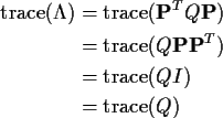
Finally, remember the properties of the trace and get
$$\begin{align*}{\rm trace}({\bf\Lambda}) & = {\rm trace}( {\bf P}^T Q{\bf P}) \\ ... ...}(Q{\bf P}{\bf P}^T) \\ & = {\rm trace}(QI) \\ & = {\rm trace}(Q) \end{align*}$$

Application to Error Sum of Squares

Recall that

$$\frac{{\rm ESS}}{\sigma^2} = (Z^*)^T (I-H) Z^*$$

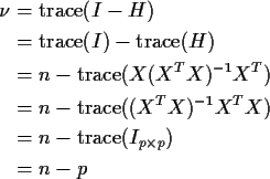
where $Z^* = \epsilon/\sigma$ is multivariate standard normal. The matrix I-H is idempotent so ${\rm ESS}/\sigma^2$ has a $\chi^2$ distribution with degrees of freedom $\nu$ equal to ${\rm trace}(I-H)$:
$$\begin{align*}\nu & = {\rm trace}(I-H) \\ & = {\rm trace}(I) - {\rm trace}(H) \... ...(X^TX)^{-1}X^TX) \\ & = n- {\rm trace}(I_{p \times p}) \\ & = n-p \end{align*}$$

Quadratic forms, Diagonalization and Eigenvalues

The function

$$f(x_1,\ldots,x_n)=f(x) = x^T Q x = \sum_{i,j} Q_{i,j} x_i x_j$$

is a quadratic form. The coefficient of a cross product term like x₁x₂ is Q_1,2+Q_2,1 so the function is unchanged if each of Q_1,2 and Q_2,1 is replaced by their average. In other words we might as well assume that the matrix Q is symmetric. Consider for example the function f(x₁,x₂) = 6x₁²+3x₂²-4x₁x₂. The matrix Q is

$$\left[\begin{array}{rr} 6 & -2 \\ -2 & 3 \end{array}\right]$$

What I did in class is the n-dimensional version of the following: Find new variables y₁ = a_1,1x₁ + a_1,2 x₂ and y₂ = a_2,1x₁+a_2,2 x₂ and constants $\lambda_1$ and $\lambda_2$such that $f(x_1,x_2) = \lambda_1 y_1^2 + \lambda_2 y_2^2$. Put in the expressions for y_i in terms of the x_i and you get

$$f(x_1,x_2) = ( \lambda_1 a_{1,1}^2 + \lambda_2 a_{2,1}^2) x_1... ...bda_1 a_{1,1}a_{1,2} + \lambda_2 a_{2,1} a_{2,2}) x_1 x_2 \, .$$

Comparing coefficients we can check that

$$Q = A^T \Lambda A$$

where A is the matrix with entries a_i,j and $\Lambda$ is a diagonal matrix with $\lambda_1$ and $\lambda_2$ on the diagonal. In other words we have to diagonalize Q.

To find the eigenvalues of Q we can solve $det(A-\lambda I) =0$The characteristic polynomial is $(6-\lambda)(3-\lambda) -4 = \lambda^2 -9\lambda+14$ whose two roots are 2 and 7. To find the corresponding eigenvectors you ``solve'' $(Q-\lambda_iI)v = 0$. For $\lambda_1 = 7$you get the equations

$$-v_1-2v_2=0 \qquad \mbox{and} \qquad -2v_1-4v_2=0$$

These equations are linearly dependent (otherwise the only solution would be v=0 and $\lambda$ would not be an eigenvalue). Solving either one gives v₁=-2v₂ so that (2,-1)^T is an eigenvector as is any non-zero multiple of that vector. To get a normalized eigenvector you divide through by the length of the vector, that is, by $\sqrt{5}$. The second eigenvector may be found similarly. We get the equation 2v₂= 4v₁ so that (1,2)^T is an eigenvector for the eigenvalue 2. After normalizing we stick these two eigenvectors in the matrix I called P obtaining

$$P=\left[\begin{array}{rr} \frac{2}{\sqrt{5}} & \frac{1}{\sqrt... ...\\ \frac{-1}{\sqrt{5}}& \frac{2}{\sqrt{5}} \end{array}\right]$$

Now check that

$$P\Lambda^T P^T = \left[\begin{array}{rr} \frac{2}{\sqrt{5}} &... ...left[\begin{array}{rr} 6 & -2 \\ -2 & 3 \end{array}\right] = Q$$

This makes the matrix A above be P^T and $y_1 = (2x_1-x_2)/\sqrt{5}$ and $y_2 = (x_1+2x_2)/\sqrt{5}$. You can check that 7y₁² + 2y₂² = 6x₁²+3x₂² -4x₁x₂ as desired.

As a second example consider a sample of size 3 from the standard normal distribution, say, Z₁, Z₂ and Z₃. Then you know that (n-1)s_Z² is supposed to have a $\chi^2$ distribution on n-1 degrees of freedom where now n=2. Expanding out

$$2s_Z^2 = (Z_1-\bar{Z})^2 + (Z_2-\bar{Z})^2 +(Z_3-\bar{Z})^2$$

we get the quadratic form

2Z₁²/3 +2Z₂²/3 + 2 Z₃²/3 -2Z₁Z₂/3 - 2 Z₁Z₃/3 -2 Z₂Z₃/3

for which the matrix Q is

$$Q = \left[\begin{array}{rrr} 2/3 & -1/3 & -1/3 \\ -1/3 & 2/3 & -1/3 \\ -1/3 & -1/3 & 2/3 \end{array}\right]$$

The determinant of $Q-\lambda I$ may be found to be $-\lambda^3 + 2\lambda^2 -\lambda$. This factors as $-\lambda(\lambda-1)^2$ so that the eigenvalues are 1, 1, and 0. An eigenvector corresponding to 0 is (1,1,1)^T. Corresponding to the other two eigenvalues there are actually many possibilities. The equations are v₁+v₂+v₃ = 0 which is 1 equation in 3 unknowns so has a two dimensional solution space. For instance the vector (1,-1,0)^T is a solution. The third solution would then be perpendicular to this, making the first two entries equal. Thus (1,1,-2)^Tis a third eigenvector.

The key point in the , however, is that the distribution of the quadratic form Z^TQZ depends only on the eigenvalues of Q and not on the eigenvectors. We can rewrite 2s_Z² in the form (Z₁^*)² + (Z₂^*)². To find Z₁* and Z₂* we fill up a matrix P with columns which are our eigenvectors, scaled to have length 1. This makes

$$P = \left[\begin{array}{rrr} \frac{1}{\sqrt{2}} & \frac{1}{\s... ...& \frac{-2}{\sqrt{6}} & \frac{1}{\sqrt{3}} \end{array}\right]$$

and we find Z^* = P^T Z to have components

$$Z_1^* = Z_1/\sqrt{2} - Z_2/\sqrt{2}$$

$$Z_2^* = Z_1/\sqrt{6} + Z_2/\sqrt{6} - 2 Z_3/\sqrt{6}$$

and

$$Z_3^* = (Z_1+Z_2+Z_3)/\sqrt{3} = \sqrt{3} \bar{Z} \,$$

You should check that these new variables all have variance 1 and all covariances equal to 0. In other words they are standard normals. Also check that (Z₁^*)² + (Z₂^*)²= 2s_Z². Since we have written 2s_Z² as a sum of square of two of these independent normals we can conclude that 2s_Z² has a $\chi_2^2$ distribution.