next up previous


Postscript version of these notes

STAT 350: Lecture 6

Reading: Chapter 7 sections 5 and 7

Polynomial Regression Continued

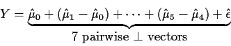
We have fitted a sequence of models to the data:

Model Model equation Fitted value
0 $Y_i = \beta_0 +\epsilon_i $ $\hat\mu_0 = \left[
\begin{array}{c} \bar{Y} \\ \vdots \\ \bar{Y}\end{array}\right]$
     
1 $Y_i = \beta_0 + \beta_1 t_i + \epsilon_i $ $\hat\mu_1 =
\left[
\begin{array}{c}
\hat\beta_0 + \hat\beta_1 t_1 \\
\vdots
\\
\\
\hat\beta_0 + \hat\beta_1 t_{n}
\end{array}\right]
$
     
$\vdots $ $\vdots $ $\vdots $
     
5 $Y_i = \beta_0 + \beta_1 t_i + +\cdots + \beta_5 t_i^5 + \epsilon_i$ $\hat\mu_5$

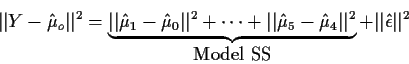
This leads to the decomposition
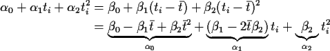
\begin{displaymath}Y=\underbrace{\hat\mu_0+(\hat\mu_1-\hat\mu_0) + \cdots + (\ha...
...\hat\mu_4) + \hat\epsilon}_{\mbox{7 pairwise $\perp$ vectors}}
\end{displaymath}

We convert this decomposition to an ANOVA table via Pythagoras:


\begin{displaymath}\vert\vert Y-\hat\mu_o\vert\vert^2 =
\underbrace{\vert\vert\...
...ert^2}_{\mbox{Model
SS}}
+ \vert\vert\hat\epsilon\vert\vert^2
\end{displaymath}

or

\begin{displaymath}\mbox{Total SS (Corrected)} = \mbox{Model SS} + \mbox{Error SS}
\end{displaymath}

Notice that the Model SS has been decomposed into a sum of 5 individual sums of squares.

Summary of points to take from example

1.
When I used SAS I fitted the model equation

\begin{displaymath}Y_i = \beta_0 + \beta_1(t_i -\bar{t}) + \beta-2 (t_i - \bar{t})^2 + \cdots
+ \beta_p (t_i-\bar{t})^p + \epsilon_i
\end{displaymath}

What would have happened if I had not subtracted $\bar{t}$? Then the entry in row i+1 and column j+1 of XTX is

\begin{displaymath}\sum_{k=1^n} t_k^{i+j}
\end{displaymath}

For instance, for i=5 and j=5 for our data we get

\begin{displaymath}(1971)^{10} +(1972)^{10} + \cdots = \mbox{HUGE}
\end{displaymath}

Most packages pronounce XTX singular. However, after recoding by subtracting $\bar{t} = 1975.5$ this entry becomes

\begin{displaymath}(-4.5)^{10}+(-3.5)^{10} + \cdots
\end{displaymath}

which can be calculated ``fairly'' accurately.

2.
Compare

\begin{displaymath}\mu_i = \alpha_0 + \alpha_1 t_i + \alpha_2 t_i^2 + \cdots +\alpha_p t_i^p
\end{displaymath}

and

\begin{displaymath}\mu_i = \beta_0 + \beta_1(t_i-\bar{t}) + \beta_2(t_i-\bar{t})^2 + \cdots +\beta_p (t_i-\bar{t})^p
\end{displaymath}

I do the case p=2 for simplicity
\begin{align*}\alpha_0 + \alpha_1 t_i + \alpha_2 t_i^2 & = \beta_0 + \beta_1(t_i...
...t} \beta_2)}_{\alpha_1} t_i +
\underbrace{\beta_2}_{\alpha_2} t_i^2
\end{align*}
So the parameter vector $\alpha$ is a linear transformation of $\beta$:

\begin{displaymath}\left[\begin{array}{c} \alpha_0 \\ \alpha_1 \\ \alpha_2 \end{...
...in{array}{c} \beta_0 \\ \beta_1 \\ \beta_2 \end{array} \right]
\end{displaymath}

It is also an algebraic fact that

\begin{displaymath}\hat\alpha = A \hat\beta
\end{displaymath}

but $\hat\beta$ suffers from much less round off error.

3.
Extrapolation is very dangerous -- good extrapolation requires models with a good physical / scientific basis.

4.
How do we decide on a good value for p? A convenient informal procedure is based on the Multiple R2 or Multiple Correlation (=R) where
\begin{align*}R^2 &= \mbox{fraction of variation of $Y$\space \lq\lq explained'' by r...
...)}
\\ & = 1 - \frac{\sum (Y_i - \hat\mu_i)^2}{\sum(Y_i -\bar{Y})^2}
\end{align*}

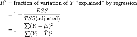
For our example we have the following results:

Degree R2
1 0.8455
2 0.9213
3 0.9922
4 0.9922
5 0.9996

Remarks:

The effect of adding variables in different orders

In class I warned that the decomposition of the Model SS depended on the order in which the variables are entered into the model in SAS. Here is a sequence of SAS runs together with the resulting ANOVA tables.

The Code from Lecture 5.

options pagesize=60 linesize=80;
data insure;
  infile 'insure.dat';
  input year cost;
  code = year - 1975.5 ;
  c2=code**2 ;
  c3=code**3 ;
  c4=code**4 ;
  c5=code**5 ;
proc glm  data=insure;
   model cost = code c2 c3 c4 c5 ;
run ;

Edited output:

Dependent Variable: COST

Source            DF        Type I SS     Mean Square   F Value     Pr > F

CODE               1     3328.3209709    3328.3209709   9081.45     0.0001
C2                 1      298.6522917     298.6522917    814.88     0.0001
C3                 1      278.9323940     278.9323940    761.08     0.0001
C4                 1        0.0006756       0.0006756      0.00     0.9678
C5                 1       29.3444412      29.3444412     80.07     0.0009

Model              5     3935.2507732     787.0501546   2147.50     0.0001
Error              4        1.4659868       0.3664967
Corrected Total    9     3936.7167600

Changing the model statement in proc glm to

   model cost =  code c4 c5 c2 c3 ;
gives
Dependent Variable: COST
                               Sum of            Mean
Source            DF          Squares          Square   F Value     Pr > F

Model              5     3935.2507732     787.0501546   2147.50     0.0001
Error              4        1.4659868       0.3664967
Corrected Total    9     3936.7167600

Source            DF        Type I SS     Mean Square   F Value     Pr > F

CODE               1     3328.3209709    3328.3209709   9081.45     0.0001
C4                 1      277.7844273     277.7844273    757.95     0.0001
C5                 1      235.9180720     235.9180720    643.71     0.0001
C2                 1       20.8685399      20.8685399     56.94     0.0017
C3                 1       72.3587631      72.3587631    197.43     0.0001

Source            DF      Type III SS     Mean Square   F Value     Pr > F

CODE               1       0.88117350      0.88117350      2.40     0.1959
C4                 1       0.00067556      0.00067556      0.00     0.9678
C5                 1      29.34444115     29.34444115     80.07     0.0009
C2                 1      20.86853994     20.86853994     56.94     0.0017
C3                 1      72.35876312     72.35876312    197.43     0.0001

                                  T for H0:    Pr > |T|   Std Error of
Parameter            Estimate    Parameter=0                Estimate

INTERCEPT         64.88753906         176.14     0.0001     0.36839358
CODE              -0.50238411          -1.55     0.1959     0.32399642
C4                -0.00020251          -0.04     0.9678     0.00471673
C5                -0.01939615          -8.95     0.0009     0.00216764
C2                 0.75623470           7.55     0.0017     0.10021797
C3                 0.80157430          14.05     0.0001     0.05704706
You will see that for CODE the SS is unchanged but after that, the SS are all changed. The MODEL, ERROR and TOTAL SS are unchanged, though. Each Type 1 SS is the sum of squared entries in the difference in two vectors of fitted values. So, e.g., the line C5 is computed by fitting the two models

\begin{displaymath}\mu_i = \beta_0 + \beta_1 t_i +\beta_4 t_i^4
\end{displaymath}

and

\begin{displaymath}\mu_i = \beta_0 + \beta_1 t_i +\beta_4 t_i^4 +\beta_5 t_i^5 \, .
\end{displaymath}

The Type I SS is the squared length of the difference between the two fitted vectors. To compute a line in the Type III sum of squares table you also compare two models, but, in this case, the two models are the full fifth degree polynomial and the model containing every power except the one matching the line you are looking at. So, for example, the C4 line compares the models

\begin{displaymath}\mu_i = \beta_0 + \beta_1 t_i +\beta_2 t_i^2 +\beta_3 t_i^3 +\beta_5 t_i^5
\end{displaymath}

and

\begin{displaymath}\mu_i = \beta_0 + \beta_1 t_i +\beta_2 t_i^2 +\beta_3 t_i^3 +\beta_4 t_i^4 +\beta_5 t_i^5 \, .
\end{displaymath}

For polynomial regression this comparison is silly; no one would expect a model like the fifth degree polynomial in which the coefficient of t4 is exactly 0 to be realistic. In many multiple regression problems, however, the type III SS are more useful.

It is worth remarking that the estimated coefficients are the same regardless of the order in which the columns are listed. This is also true of type III SS. You will also see that all the F P-values with 1 df in the type III SS table are matched by the corresponding P-values for the t tests.


next up previous


Richard Lockhart
1999-01-12